How to Measure Canopy Stomatal Conductance.
Canopy stomatal conductance is a measure of water vapour transfer from the plant to the atmosphere. How to measure canopy stomatal conductance is explained in this article along with methods, equations and statistics on its analysis.
Conductance is the ease with which water can transfer from the plant to the atmosphere with higher values indicating easier transfer. Canopy conductance is a fundamental parameter in plant hydraulics and its understanding is important for plant water relations.
Canopy conductance (denoted by Gc or Gt) and canopy stomatal conductance (denoted by Gs) are often used interchangeably but have the same definition and methodology. Canopy stomatal conductance is measured via sap flow sensors and integrates water flux of the entire canopy. In contrast, stomatal conductance, or leaf stomatal conductance, is a leaf level measurement of conductance and is typically measured with a porometer (e.g. SC-1 leaf porometer) and is usually denoted with the symbol gs.
Why is canopy conductance important?
Canopy conductance measurements can be used to understand plant physiology, water relations and hydraulic architecture. Canopy conductance can also be used to gain insights into energy exchanges between vegetation and the atmosphere as well as to identify ecological interactions and evolutionary adaptations.
The inverse of conductance is resistance. Therefore, knowledge about canopy conductance can be used to gain insights into resistance of water flow within and from plants. The most important variable influencing canopy resistance is stomatal opening where open stomata offer less resistance and partially closed stomata creating higher resistance.
Canopy conductance is useful for understanding the hydrologic cycle as well as energy exchanges between vegetation and the atmosphere. Canopy conductance fr

om sap flow measurements is routinely used in combination with Eddy Correlation techniques to understand water vapour exchanges between vegetation and the atmosphere.
Canopy conductance and resistance can also be used to compare species hydraulic architecture. For example, the canopy conductance of coexisting species within a habitat, or phylogenetic independent contrasts (PIC) between closely related species, can be compared to gain insights into the ecological and evolutionary significance of varying hydraulic architecture. Differences in canopy conductance or resistance will likely reflect evolutionary adaptations of the hydraulic pathways within the plant (e.g. xylem diameter, xylem length, xylem density, stomatal density, wood density, and more). Therefore, accurate measurements of canopy conductance is useful for plant physiologist and evolutionary biologists.
Required equipment to measure canopy conductance.
An Implexx Sap Flow Sensor and an ATMOS 41 Weather Station is required to measure canopy conductance.
The Implexx Sap Flow Sensor is needed to measure water (sap) flux within the plant.
The Implexx Sap Flow Sensor is installed on the trunk or stem of the plant or tree. Typically, the sensor is installed lower on the trunk beneath the crown. However, some experiments or hypotheses may test canopy conductance at various locations along the trunk such as upper versus lower branches or northern versus southern aspects.
The ATMOS 41 Weather Station is needed to measure atmospheric evaporative demand variables including vapour pressure deficit (VPD), wind, solar radiation, temperature, and relative humidity.
The weather station should be installed as close as possible to the measured plants while still following standard protocols on where to install a weather station (i.e. in the open and away from obstructions).
Canopy conductance calculated with an inverse Penman-Monteith equation.
Paudel et al (2015) proposed a method to calculate canopy conductance using an inverse Penman-Monteith evapotranspiration equation. The following equation was proposed by Paudel et al (2015) to calculate canopy conductance (Gc):
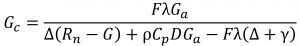
where F is sap flux density (kg m−2 s−1) measured with the Implexx Sap Flow Sensor, λ is the latent heat of vaporization of water (J kg−1), Ga is canopy aerodynamic resistance (m s−1), Δ is the slope of the relationship between water vapor pressure and temperature [KPa °C−1], ρ is the density of dry air (kg m−3)], Cp is specific heat of dry air at constant pressure (J kg−1 C−1), D is vapor pressure deficit (KPa), γ is the psychrometric constant (KPa °C−1), Rn is net radiation (MJ m−2 s−1) and G is soil heat flux (MJ m−2 s−1).
Here is how to calculate all the parameters in the canopy conductance equation:
- F – use data measured from an Implexx Sap Flow Sensor. Note that F is sap flux density which is kg of sap per m2 of sapwood area per second. The Implexx Sap Flow Sensor outputs total sap flow (kg per hour) and this will need to be converted to F.
- λ =1000000*(2.5-(0.00236*T)) where T is air temperature (°C) measured by the ATMOS 41 weather station.
- Ga = 0.1*u where is wind speed (m s−1) measured by the ATMOS 41 Weather Station.
- Δ =((λ/1000)*Mw*eo)/(0.00813*(T+273)*(T+273))/(1000)
- Mw = molecular weight of water and is a constant value of 18.
- eo = saturated vapour pressure (kPa) =0.6108*EXP((17.27*T)/(T+237.3))
- Rn – it is possible to use the solar radiation measurement from the ATMOS 41 Weather Station. Check the units of measurement, though, as most pyranometers measure in units W m−2. There are many other methods to measure net radiation with other sensors, if required.
- G – soil heat flux can be measured with a sensor. Often, G is negligible, and it is conveniently given a value of 0 or is ignored.
- ρ is a constant value of 1.204.
- Cp is a constant value of 1010.
- D =(610.8*EXP(17.29*T/(T+237.3))/1000)*(1-RH) where RH is relative humidity and is measured with the ATMOS 41 Weather Station.
- γ is a constant value of 0.0667.
Canopy conductance of the “average” stomata.
Köstner proposed a method to calculate the canopy conductance of the “average” stomata across the entire canopy (Köstner et al 1992, 1996, 2001). Total water vapour transfer conductance (Gt) is defined as:
Gt = (Gv*TK)*(Ec/D)
where:
- Gv is the gas constant of water vapour and is a constant value of 0.462 (m3 kPa−1 kg−1 K−1).
- TK is air temperature in Kelvins (i.e. T + 273.15 where T is air temperature measured by the ATMOS 41 Weather Station).
- Ec is canopy water flux (kg m−2 s−1) calculated as total tree sap flow, measured from the Implexx Sap Flow Sensor (l/h) divided by canopy projection area (m2) per second. Note that Ec is different to F as Ec is corrected for canopy projection area whereas F is corrected for sapwood area.
- D is vapour pressure deficit (kPa) =(610.8*EXP(17.29*T/(T+237.3))/1000)*(1-RH) where RH is relative humidity and is measured with the ATMOS 41 Weather Station.
- Köstner et al (1992, 2001) noted that the Gc is related to Gt by subtracting Ga, defined as: 1/Gc = 1/Gt – 1/Ga
Interpretation of data.
Researchers must carefully decide whether Gc or Gt, or both, is more appropriate parameter for their experiment and hypotheses. The interpretation of results will likely differ depending on whether data has been analysed via the Gc or Gt equation. As an example, below is presented a data set from 30 days of measurement for a 1.5m tall, potted, lilly pilly (Syzygium paniculatum Gaertn.) sapling growing in a common garden, Melbourne, Australia during summer. The data set includes sap flow measured with the Implexx Sap Flow Sensor, weather data measured via the ATMOS 41 Weather Station, and Gc and Gt calculated via the above equations.
Figure 1 is an example set of data over 7 days for sap flow, Gc and Gt. All variables show a cycle where maximums occur during the day and minimums at night. However, there are differences when maximums occur during the day. During the night, Gc is consistently low or zero whereas sap flow is relatively high during the early night and Gt is relatively high during the latter portion of the night. These differences may be related to physiological processes such as stem refilling or nocturnal transpiration. However, further measurements and analysis are required for a better understanding.
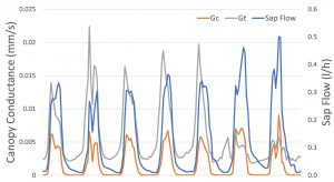
Figure 1. An example data set of 7 days of sap flow (blue), and canopy conductance calculated by evapotranspiration equation (Gc, orange) or Köstner equation (Gt, grey).
The relationship between Gc, Gt and atmospheric variables may also lead to difference in data interpretation. For example, Figure 2 shows the relationship between VPD, Gc and Gt. Figure 2A shows no relationship between VPD and Gc; whereas Figure 2B shows a negative relationship between VPD and Gt. Careful consideration of the Gc and Gt equation is required for appropriate interpretation of these results.
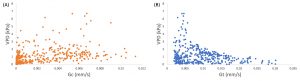
Figure 2. The relationship between VPD and canopy conductance calculated with the evapotranspiration equation (A, orange) or Köstner equation (B, blue).
Conversely, the relationship between Gc, Gt and solar radiation yields a different interpretation. Figure 3A is the correlation between solar radiation (daytime only) and Gc with a positive linear relationship. Figure 3B is the relationship between solar radiation (daytime only) and Gt with no relationship.
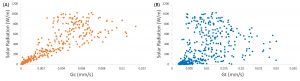
Figure 3. The relationship between solar radiation and canopy conductance calculated via the evapotranspiration equation (A, orange) or Köstner equation (B, blue).
Although these examples and analyses are simple, and more data is required for a comprehensive interpretation, it does emphasise that care needs to be exercised when choosing canopy conductance methods. The most appropriate method, with the correction interpretation, is required for a rigorous and thorough analysis.
References.
Köstner et al 1992. Oecologia 91, 350-359. https://www.jstor.org/stable/4220079
Köstner et al 1996. Theoretical and Applied Climatology 53, 105-113. https://link.springer.com/article/10.1007/BF00866415
Köstner 2001. Meteorology and Atmospheric Physics 76, 69-82. https://link.springer.com/article/10.1007/s007030170040
Pauldel et al 2015. Tree Physiology 35, 425–438. doi:10.1093/treephys/tpu113